지도학습 | 분류용 선형 모델 (Linear Classification Model)

선형 모델은 Classification 문제에도 많이 사용된다. 먼저, binary classification을 살펴보자. 수식은 다음과 같다.

y = w0⋅x0 + w1⋅x1 + ... + wp⋅xp + b > 0

 

가장 널리 알려진 두 개의 선형 알고리즘은 Logistic Regression(회귀 알고리즘이 아니다)과 Support Vector Machine(LinearSVC)이다. forge 데이터셋을 사용해서 LogisticRegression과 LinearSVC 모델을 만들고, 이 모델이 만든 결정경계를 그림으로 나타내보자.

 

# !pip install mglearn
import mglearn
from sklearn.linear_model import LogisticRegression
from sklearn.svm import LinearSVC
import matplotlib.pyplot as plt

# Loading dataset
X, Y = mglearn.datasets.make_forge()

# Creating subplot
fig, axes = plt.subplots(1, 2, figsize=(10, 3))

for model, ax in zip([LinearSVC(max_iter=5000), LogisticRegression()], axes):
    clf = model.fit(X, Y)  # Instantiate and fit the model
    mglearn.plots.plot_2d_separator(clf, X, fill=False, eps=0.5, ax=ax, alpha=0.7)
    mglearn.discrete_scatter(X[:, 0], X[:, 1], Y, ax=ax)  # Corrected to Y

# Adding a legend to the first subplot
axes[0].legend(["Class 0", "Class 1"], loc="best")
plt.show()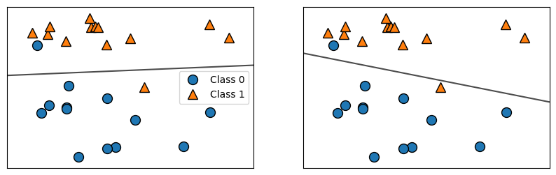

 

 

두 모델이 거의 비슷한 결정 경계(Decision Boundry)를 만들었다. 그리고 같은 포인트 두개도 잘못 분류했다. Ridge와 마찬가지로, 이 두 모델은 L2 규제를 사용한다. 이 규제, regulation의 강도를 결정하는 매개변서는 C인데, 이 C값이 높아지면 규제가 감소한다. 즉, C를 높은 값으로 지정하면, 훈련 세트에 가능한 최대로 맞추게 되고 (과대적합이 될 수 있다), 반면에 C를 낮추면 weight(w)값이 0에 가까워진다. C의 값에 따라 어떻게 그려지는지 보자.

 

mglearn.plots.plot_linear_svc_regularization()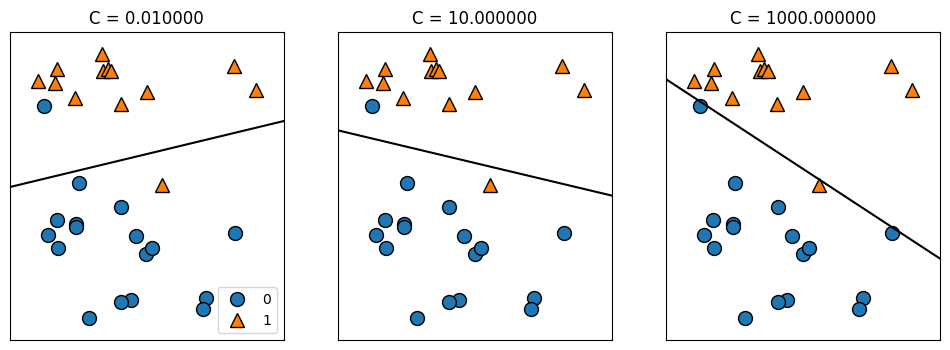

 

 

C가 0.01일 때, 많은 규제가 적용되었다. 오른쪽으로 갈수록 규제가 커졌는데, 두 샘플(파란 동그라미)때문에 민감해져서 결정결계가 많이 기울었다. 여전히 하나는 잘 분류가 안되었지만, 0.01때, 10일때에 비해 분류를 조금 더 정밀하게 해내었다.

 

Regression(회귀)와 비슷하게, 선형 모델이 직선이어서 너무 제한적인 것처럼 보이지만, 고차원에서는 매우 강력해진다. 유방암 데이터셋을 사용해 LogisticRegression을 좀 더 자세히 분석해보자.

 

from sklearn.datasets import load_breast_cancer

cancer = load_breast_cancer()

X_train, X_test, Y_train, Y_test = train_test_split(
    cancer.data, cancer.target, stratify=cancer.target, random_state=42
)

logreg = LogisticRegression(max_iter=5000).fit(X_train, Y_train)

print("training score: {:.3f}".format(logreg.score(X_train, Y_train)))
print("testing score: {:.3f}".format(logreg.score(X_test, Y_test)))

training score: 0.958
testing score: 0.958

 

기본값 C=1이 훈련세트, 테스트세트 양쪽 모두 거의 96%정확도를 보여주면서 아주 훌륭한 성능을 냈다. 하지만, 훈련 세트와 테스트 세트의 성능이 매우 비슷하기때문에, 과소적합으로 보인다. 모델의 제약을 조금 풀어주기 위해, C를 증가시켜봤다.

logreg100 = LogisticRegression(C=100, max_iter=5000).fit(X_train, Y_train)

print("training score: {:.3f}".format(logreg100.score(X_train, Y_train)))
print("testing score: {:.3f}".format(logreg100.score(X_test, Y_test)))

training score: 0.981
testing score: 0.965

 

훈련세트와 테스트세트의 정확도도 높아졌다. 복잡도가 높은 모델일수록 성능이 좋아짐을 말해준다. 이번엔 규제를 더 강하게 하기 위해, C를 0.01로 낮춰보자.

logreg001 = LogisticRegression(C=0.01, max_iter=5000).fit(X_train, Y_train)

print("training score: {:.3f}".format(logreg001.score(X_train, Y_train)))
print("testing score: {:.3f}".format(logreg001.score(X_test, Y_test)))

training score: 0.953
testing score: 0.951

 

훈련세트와 테스트 세트의 정확도가 기본 1일때보다 낮아진다. 그러면 이렇게 설정을 다르게 했을 때, 계수의 크기를 살펴보자.

plt.plot(logreg100.coef_.T, '^', label="C=100")
plt.plot(logreg.coef_.T, 'o', label="C=1")
plt.plot(logreg001.coef_.T, 'v', label="C=0.01")

plt.xticks(range(cancer.data.shape[1]), cancer.feature_names, rotation=90)
xlims = plt.xlim()
plt.hlines(0, xlims[0], xlims[1])
plt.xlim(xlims)
plt.ylim(-5, 5)

plt.legend()

 

 

모델이 몇개 안되는 특성만 사용하겠지만, 더 이해하기 쉬운 모델이 필요하면 L1규제를 사용하는것이 좋다. 다음은 L1을 사용하는 예시다.

for C, marker in zip([0.001, 1, 100], ['o', '^', 'v']):
  lr_l1 = LogisticRegression(solver='liblinear', C=C, penalty='l1', max_iter=1000).fit(X_train, Y_train)
  print("C={:.3f} L1 Logistic Regression Training Score : {:.2f}".format(C, lr_l1.score(X_train, Y_train)))
  print("C={:.3f} L1 Logistic Regression Testing Score : {:.2f}".format(C, lr_l1.score(X_test, Y_test)))

  plt.plot(lr_l1.coef_.T, marker, label="C={:.3f}".format(C))

plt.xticks(range(cancer.data.shape[1]), cancer.feature_names, rotation=90)
xlims = plt.xlim()
plt.hlines(0, xlims[0], xlims[1])
plt.xlim(xlims)
plt.xlabel("Feature")
plt.ylabel("Coefficient Size")

plt.ylim(-5, 5)
plt.legend(loc=3)

C=0.001 L1 Logistic Regression Training Score : 0.91
C=0.001 L1 Logistic Regression Testing Score : 0.92
C=1.000 L1 Logistic Regression Training Score : 0.96
C=1.000 L1 Logistic Regression Testing Score : 0.96
C=100.000 L1 Logistic Regression Training Score : 0.99
C=100.000 L1 Logistic Regression Testing Score : 0.98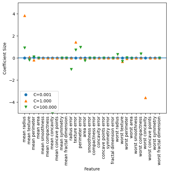

L1 규제를 사용했을 때, C가 높아질수록 테스트나 트레이팅 세트 점수가 상승했다. 

 

Reference

https://colab.research.google.com/drive/1fzSiPpwbTUplw6G0PJSpGaVBWx5CEMIZ?usp=sharing

_02_supervised_machine_learning.ipynb

https://www.yes24.com/Product/Goods/42806875

파이썬 라이브러리를 활용한 머신러닝 - 예스24